

How To Filter Email Addresses In Excel
Author: Oscar Cronquist Article last updated on February 01, 2019
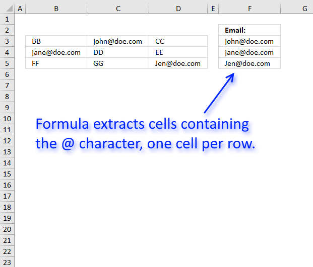
Question: How to excerpt email addresses from this canvas? (Encounter film below)
Answer:
It depends on how the emails are populated in your worksheet?
- Are they in a unmarried cell each?
- Are there other text strings in the cell too?
Case one,
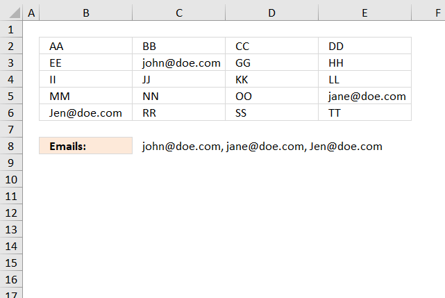
The following formula works if a jail cell contains only an email accost, meet image above. The TEXTJOIN part extracts all emails based on if character @ is found in the cell.
Array formula in cell C8:
=TEXTJOIN(", ", Truthful, IF(ISERROR(SEARCH("@", B2:E6)), "", B2:E6))
Case 2,
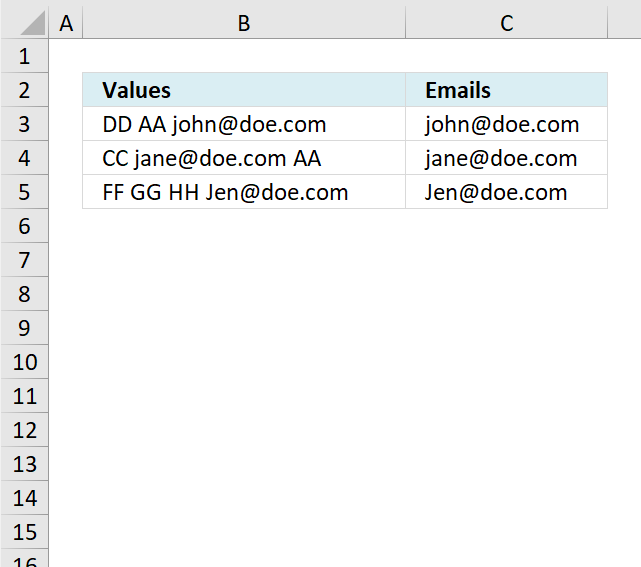
The case in a higher place has multiple text strings in each cell separated by a bare, the formula is only capable of extracting one email accost per cell and if the delimiting graphic symbol is a bare (space). You can change the formula to use any delimiting character, nevertheless, simply i delimiting character per formula.
Formula in jail cell C3:
=TRIM(MID(SUBSTITUTE(TRIM(B3), " ", REPT(" ", 200)), (LEN(LEFT(B3, SEARCH("@", B3)))-LEN(SUBSTITUTE(LEFT(B3, SEARCH("@", B3))," ", "")))*200+1, 200))
Example 3,
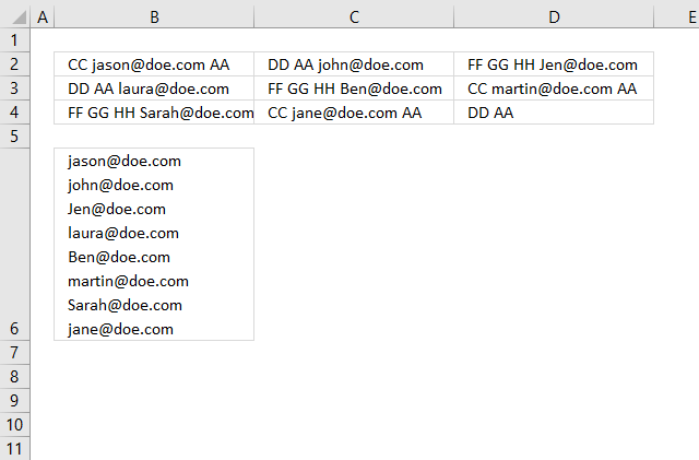
It is possible to combine the array formulas in example 1 and ii, unfortunately, the formula can still but extract one email accost per cell.
Array formula in cell B6:
=TEXTJOIN(CHAR(10), TRUE, IF(ISERROR(SEARCH("@", B2:D4)), "", TRIM(MID(SUBSTITUTE(TRIM(B2:D4), " ", REPT(" ", 200)), (LEN(LEFT(B2:D4, SEARCH("@", B2:D4)))-LEN(SUBSTITUTE(LEFT(B2:D4, SEARCH("@", B2:D4)), " ", "")))*200+1, 200))))
Cell B6 has "Wrap text" enabled, select jail cell B6 and press CTRL + 1 to open the "Format Cells" dialog box.

Example 4,
If you demand an fifty-fifty better faster formula I recommend using a UDF:
Filter words containing a given cord in a cell range [UDF]
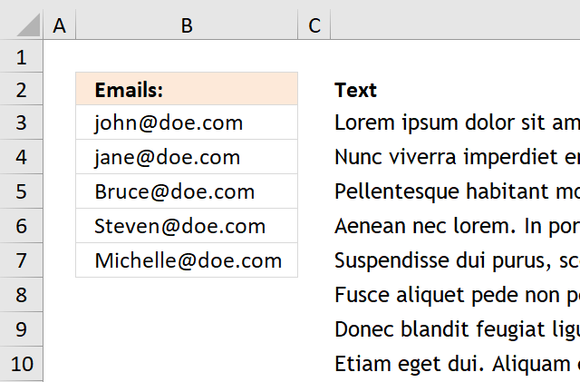
Example v,
The formula in prison cell F3 gets but one email address per row so it is very basic, however, check out the comments for more than advanced formulas.
If the cell contains an email address and also other text strings information technology won't excerpt the e-mail only, as I said, it is a very bones formula.
Assortment formula in F3:
=Index(B3:D3, i, MIN(IF(ISERROR(SEARCH("@", B3:D3)), "", MATCH(Column(B3:D3), COLUMN(B3:D3)))))
To enter an array formula, type the formula in cell F3 and then press and hold CTRL + SHIFT simultaneously, now printing Enter once. Release all keys.
 The formula bar now shows the formula with a beginning and ending curly bracket telling you that you entered the formula successfully.
Don't enter the curly brackets yourself, they appear automatically.
This article demonstrates how to filter emails with a custom part:
Filter words containing a given string in a cell range [UDF]
Explaining formula in cell F3
Pace 1 - Expect for @ character in jail cell range
The SEARCH office allows you lot to detect the grapheme position of a substring in a text string, we are, however, not interested in the position only if it exists or not in the prison cell.
SEARCH("@", B3:D3))
becomes
SEARCH("@", {"BB","[e-mail protected]","CC"}))
and returns {#VALUE!,5,#VALUE!}. This tells united states that the second value in the array contains a @ graphic symbol on position 5.
Step 2 - Convert array to TRUE or Fake
The IF role can't handle mistake values in the logical expression and then nosotros must first convert the assortment to boolean values. The ISERROR function returns TRUE if the value is an fault value and FALSE if not.
ISERROR(SEARCH("@", B3:D3))
becomes
ISERROR({#VALUE!,5,#VALUE!})
and returns {TRUE,FALSE,TRUE}.
Step 3 - Render column number if value is non an error value
IF(ISERROR(SEARCH("@", B3:D3)), "", MATCH(Cavalcade(B3:D3), Cavalcade(B3:D3)))
becomes
IF({TRUE,FALSE,True}, "", Friction match(COLUMN(B3:D3), COLUMN(B3:D3)))
To create an assortment from ane to n I use the Lucifer function and COLUMN function.
IF({True,FALSE,Truthful}, "", Lucifer(COLUMN(B3:D3), Column(B3:D3)))
becomes
IF({TRUE,FALSE,Truthful}, "", Match({two,3,4}, {2,3,iv}))
becomes
IF({TRUE,FALSE,True}, "", {1, 2,iii})
and returns {"", two,""}
Step 4 - Return the smallest column number
The MIN function calculates the smallest number in cell range or array.
MIN(IF(ISERROR(SEARCH("@", B3:D3)), "", MATCH(Cavalcade(B3:D3), Column(B3:D3))))
becomes
MIN({"", 2,""})
and returns 2.
Step iv - Return value corresponding to cavalcade number
The Alphabetize function returns a value based on a row and/or cavalcade number.
INDEX(B3:D3, MIN(IF(ISERROR(SEARCH("@", B3:D3)), "", MATCH(Cavalcade(B3:D3), COLUMN(B3:D3)))))
becomes
Index(B3:D3, two)
and returns "[email protected]".
Get Excel *.xlsx file
extract_email_2.xlsx
Learn to use regular expressions and filter emails:
Extract cell references from a formula
Learn how to use the LIKE operator to filter emails:
How to use the LIKE OPERATOR
The LIKE operator allows you to friction match a cord to a design using Excel VBA. The image above demonstrates a […]
How to use the LIKE OPERATOR

How To Filter Email Addresses In Excel,
Source: https://www.get-digital-help.com/how-to-extract-email-addresses-from-a-excel-sheet/
Posted by: beasleydody1988.blogspot.com
0 Response to "How To Filter Email Addresses In Excel"
Post a Comment